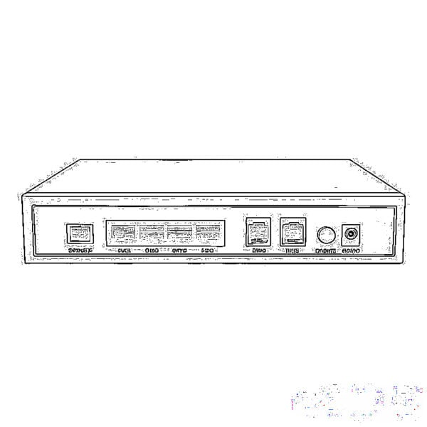


In the complex architecture of modern communication networks, switches act as crucial hubs for data transmission. Among their various components, optical modules and optical interfaces are vital for enabling high – speed and reliable data exchange. A comprehensive understanding of Switch Optical Modules, Optical Interface Types, and Fiber Optic Connectors is essential for network engineers, technicians, and anyone involved in network design, deployment, and maintenance.
Introduction
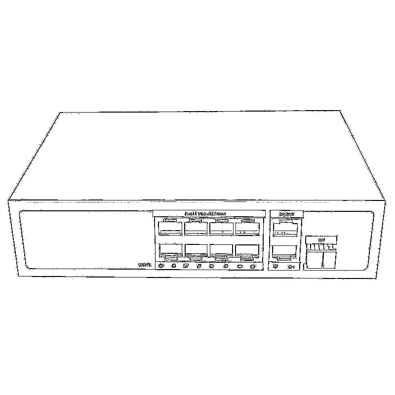
The performance of a network is heavily dependent on the efficiency of its data transmission components. Switch optical modules, which convert electrical signals to optical signals and vice – versa, and optical interfaces, which serve as the physical connection points, play a pivotal role in determining the speed, distance, and reliability of data transmission.
Common optical module types such as SFP, GBIC, XFP, and XENPAK, along with optical interfaces like FC, SC, and LC, each have their unique characteristics that make them suitable for specific application scenarios. Whether it’s a small – scale local area network (LAN) or a large – scale wide area network (WAN), choosing the right combination of optical modules and interfaces is key to ensuring optimal network performance.
Table of Contents
- Analysis of Common Optical Modules for Switches
- Optical Interface Types and Fiber Optic Connectors
- Fiber Optic Transmission Basics and Interface Adaptation
- Optical Port Working Modes and Negotiation Mechanisms
- Emerging Technology Extensions
- Selection and Maintenance Recommendations
- FAQs
Analysis of Common Optical Modules for Switches
SFP Modules
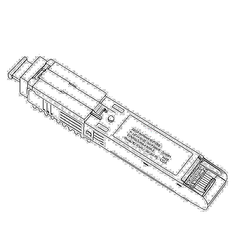
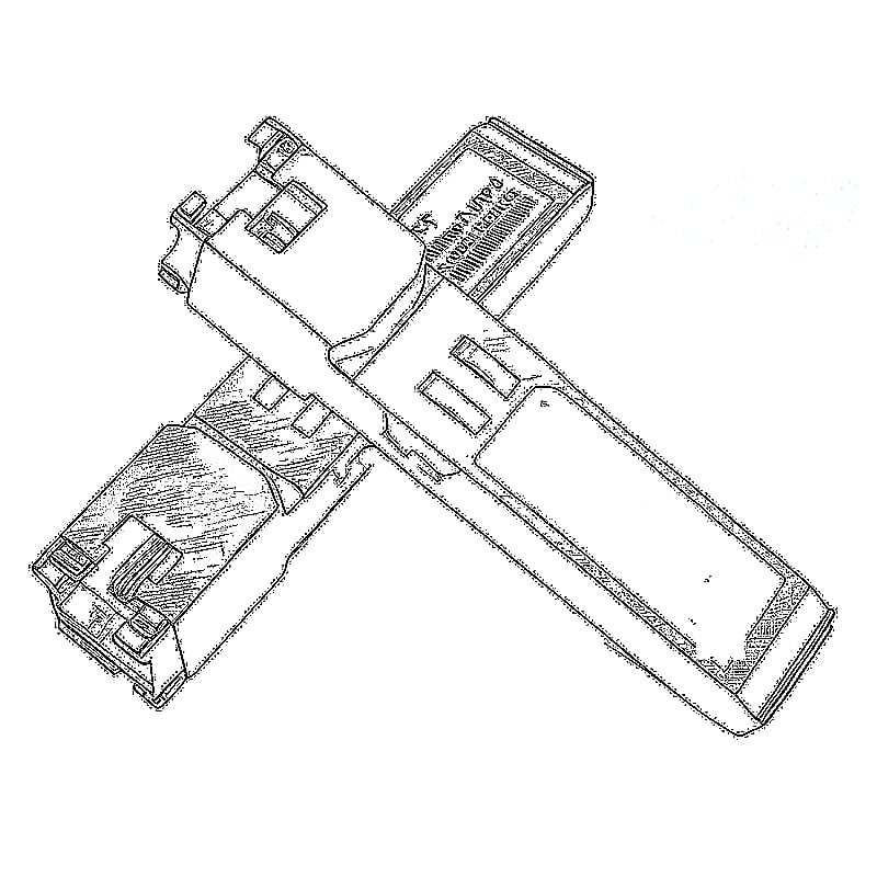
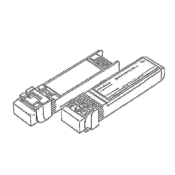
Small Form – factor Pluggable (SFP) modules are widely used in modern switches due to their compact size. Their small form factor allows for higher port density on switches, meaning more modules can be installed in the same physical space compared to larger modules. This is a significant advantage in data centers and other environments where space is at a premium.
One of the key technical differences between SFP modules and GBIC modules is their size. SFP modules are about half the size of GBIC modules, making them more suitable for high – density applications. Additionally, SFP modules support hot – swap functionality, which allows them to be inserted or removed from a switch while it is still powered on. This feature greatly simplifies maintenance and upgrades, as there is no need to power down the entire switch, minimizing network downtime.

GBIC Modules
Gigabit Interface Converter (GBIC) modules were once the standard for gigabit Ethernet connections. They are larger in size compared to SFP modules but also support hot – swap, enabling easy replacement and maintenance.
However, with the emergence of SFP modules, the market application of GBIC modules has gradually declined. They are still found in some older network equipment, but new deployments typically favor SFP modules due to their superior port density and smaller size.

XFP/XENPAK Modules
XFP and XENPAK modules are designed for 10 – gigabit data transmission. XFP modules are smaller than XENPAK modules, offering better port density. XENPAK modules, on the other hand, were one of the early 10 – gigabit module standards but have been largely replaced by XFP and other smaller form – factor modules.
XFP modules are suitable for a wide range of 10 – gigabit applications, including data center interconnects and high – speed LANs. XENPAK modules, while less common today, can still be found in some legacy 10 – gigabit networks.

Technical Evolution
The evolution of optical modules has been driven by the need for higher port density and better performance. From the larger GBIC modules to the smaller SFP modules, the trend towards miniaturization has allowed switches to support more ports without increasing their physical size. This has been crucial in meeting the growing demand for high – speed data transmission in modern networks.
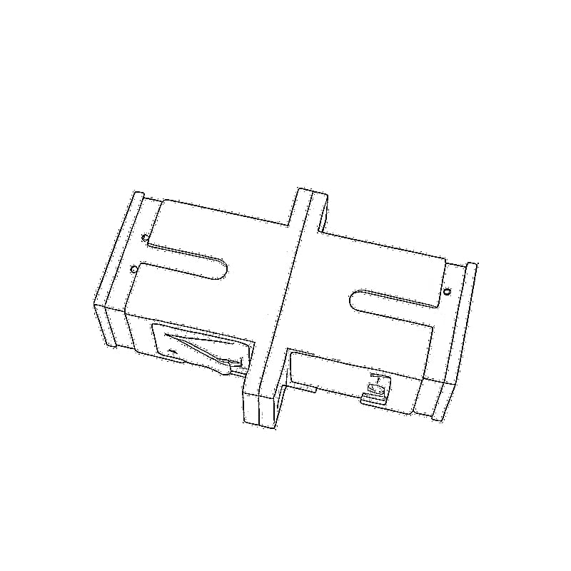
Optical Interface Types and Fiber Optic Connectors
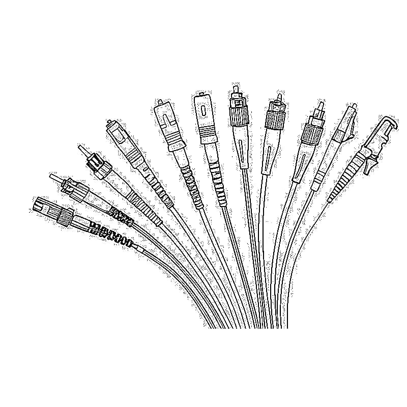
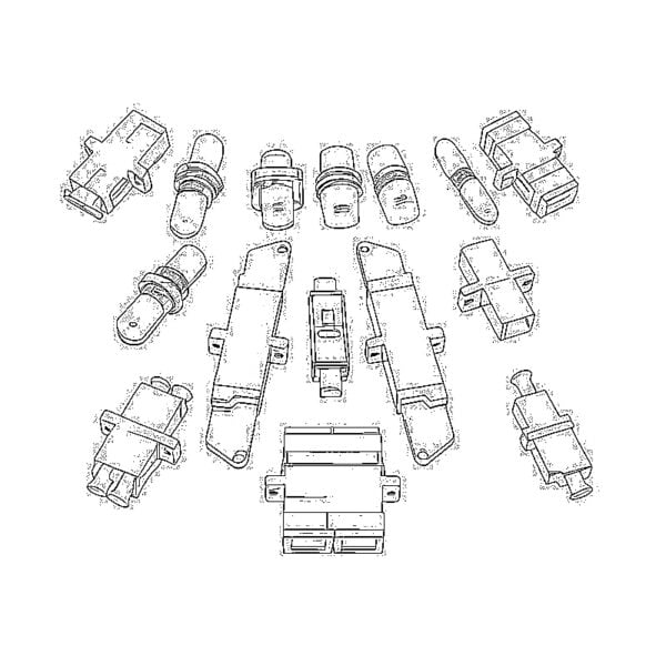
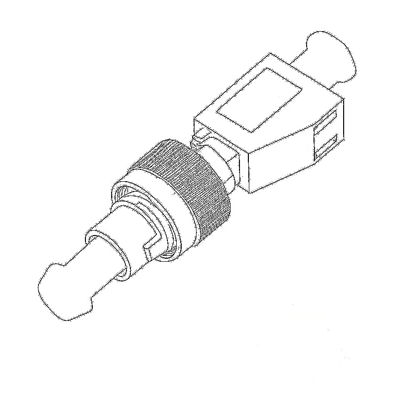
FC/SC/LC/ST Interfaces
Different optical interfaces have distinct locking mechanisms and physical structures that make them suitable for various applications.
FC interfaces use a threaded locking mechanism, which provides a secure connection. This makes them ideal for scenarios where frequent plugging and unplugging is required, such as in equipment room distribution frames, as the threaded design ensures a stable connection even after multiple insertions and removals.
SC interfaces feature a plug – in design, which is simple to use. They are commonly found in low – end Ethernet devices, such as 100Base – FX switches, due to their ease of installation and cost – effectiveness.
LC interfaces are miniaturized plug – in interfaces. Their small size makes them perfect for high – density scenarios, such as in SFP modules and data center cabling, where maximizing port density is essential.
ST interfaces use a bayonet locking mechanism, which is easy to operate with one hand. They were once widely used in fiber optic networks but have become less common in modern high – density environments.

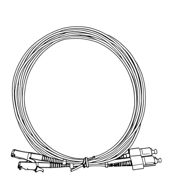
Adaptation Relationship Between Fiber Optic Connectors and Modules
There is a specific adaptation relationship between fiber optic connectors and optical modules. For example, SFP modules commonly use LC connectors, while GBIC modules typically use SC connectors. This relationship is determined by the design of the modules and the need for compatibility with different network equipment.
Key Points for Interface Selection
When selecting an optical interface, several factors need to be considered. The plug – in life of the interface is important, especially in environments where frequent connections and disconnections occur. Interfaces with a longer plug – in life will reduce the need for replacement and maintenance.
The material of the ferrule, whether ceramic or plastic, also affects the stability of the connection. Ceramic ferrules offer better precision and durability, resulting in lower insertion loss and better signal transmission. Plastic ferrules are less expensive but may not provide the same level of performance as ceramic ones in high – speed or long – distance applications.
Fiber Optic Transmission Basics and Interface Adaptation
Single – mode/Multi – mode Fibers
Single – mode and multi – mode fibers differ in core diameter, which affects their transmission characteristics. Single – mode fibers have a core diameter of 8 – 10μm, while multi – mode fibers have a core diameter of either 50μm or 62.5μm.
The wavelength of the light used in the fiber also plays a role in transmission distance. Single – mode fibers commonly use wavelengths of 1310nm and 1550nm, which allow for longer transmission distances. Multi – mode fibers typically use an 850nm wavelength, which is suitable for shorter distances.

Matching Principles Between Optical Modules and Fibers
It is essential to match the correct optical module with the appropriate fiber type. Multi – mode optical modules should be used with multi – mode fibers (typically at 850nm wavelength), and single – mode optical modules should be paired with single – mode fibers (at 1310nm or 1550nm wavelengths). Using the wrong combination can result in significant signal loss and poor network performance.

Transmission Loss Data
Transmission loss is a critical parameter in fiber optic networks. 850nm multi – mode fiber has a loss of approximately 3.0dB/km, while 1550nm single – mode fiber has a much lower loss of around 0.2dB/km. This difference in loss explains why single – mode fibers are preferred for long – distance transmission, as they can carry signals over much greater distances with minimal attenuation.

Optical Port Working Modes and Negotiation Mechanisms
Gigabit Optical Port Modes
Gigabit optical ports operate in two main modes: auto – negotiation and forced mode.
Auto – negotiation mode uses a /C/ code stream to exchange information between two connected devices. This allows the devices to automatically determine the highest common speed and duplex mode they both support, ensuring optimal performance.
Forced mode uses an /I/ code stream and manually sets the speed and duplex mode of the port. This mode is useful in situations where auto – negotiation fails or when a specific configuration is required.
Handling Negotiation Abnormalities
Negotiation abnormalities can occur when one end of a connection is in auto – negotiation mode and the other is in forced mode. In such cases, the auto – negotiation end will typically be in a DOWN state because it does not receive an acknowledgment from the forced mode end.
To resolve this issue, it is necessary to ensure that both ends are set to the same mode. If both ends are set to auto – negotiation, they will exchange /C/ code streams and establish a connection once they match on speed and duplex mode. If both ends are set to forced mode with the same speed and duplex settings, they will communicate using /I/ code streams and the connection will be UP.
Full – Duplex/Half – Duplex Modes
The 802.3 specification defines the range of speed and duplex modes supported by Ethernet interfaces. Full – duplex mode allows for simultaneous transmission and reception of data, doubling the effective bandwidth compared to half – duplex mode, which only allows one – way transmission at a time. Most modern network devices support full – duplex mode, which is essential for high – speed data transmission.
Emerging Technology Extensions
CWDM/DWDM Technologies
Coarse Wavelength Division Multiplexing (CWDM) and Dense Wavelength Division Multiplexing (DWDM) are technologies that allow multiple optical signals to be transmitted over a single fiber by using different wavelengths.
CWDM uses a wavelength spacing of 20nm, with channels ranging from 1271nm to 1611nm, totaling 18 channels. It is a cost – effective solution for medium – and short – distance capacity expansion, as it does not require expensive wavelength control devices.
DWDM uses much smaller wavelength spacing, typically between 0.4nm and 1.6nm, allowing for a much higher number of channels. This makes it suitable for long – distance, high – density bandwidth scenarios, such as backbone networks, where maximizing fiber utilization is crucial.
In terms of cost, CWDM is generally cheaper than DWDM due to its simpler technology and less stringent component requirements.
Advantages of Hot – Swap for Optical Modules
Hot – swap functionality, which allows optical modules to be inserted or removed while the switch is powered on, offers significant advantages in terms of maintenance and upgrades. It enables network administrators to replace faulty modules or upgrade to higher – performance modules without disrupting network operations, minimizing downtime and ensuring continuous network availability. This is particularly important in data centers and other critical network environments where even a short period of downtime can have significant consequences.
Selection and Maintenance Recommendations
Module and Interface Matching Table
To ensure optimal performance, it is important to select the right combination of optical modules and interfaces based on speed and transmission distance.
For gigabit speed and short – range transmission (up to a few hundred meters), SFP modules with LC interfaces paired with multi – mode fiber are a good choice.
For gigabit speed and long – range transmission (several kilometers), SFP modules with LC interfaces and single – mode fiber are suitable.
For 10 – gigabit speed and short – range applications, XFP modules with LC interfaces and multi – mode fiber can be used.
For 10 – gigabit speed and long – range transmission, XFP modules with LC interfaces and single – mode fiber are appropriate.
Troubleshooting Directions
Common problems with optical modules and interfaces include interface contamination, excessive fiber loss, and mode mismatch.
Interface contamination can occur due to dust or debris on the ferrule, leading to increased signal loss. Regular cleaning of the interfaces using appropriate cleaning tools can resolve this issue.
Excessive fiber loss can be caused by poor fiber connections, damaged fibers, or using the wrong type of fiber for the transmission distance. Testing the fiber with an optical power meter can help identify the source of the loss, and replacing damaged components or using the correct fiber type can restore performance.
Mode mismatch, which happens when a single – mode module is used with multi – mode fiber or vice versa, can result in severe signal degradation. Ensuring that the module and fiber types are matched correctly is essential to avoid this problem.
FAQs
- What is the difference between SFP modules and GBIC modules?
SFP modules are a miniaturized upgraded version of GBIC modules, with a 50% reduction in volume. They support the same functions as GBIC modules but offer higher port density, allowing twice as many ports to be deployed on the same panel. GBIC is an early gigabit interface standard and is gradually being replaced by SFP modules, although some older devices still use GBIC modules.
- How to distinguish between single – mode and multi – mode fibers?
- Color: The outer sheath of single – mode fiber is yellow, while that of multi – mode fiber is orange – red.
- Core Diameter: Single – mode fiber has a core diameter of 8 – 10μm, and multi – mode fiber has a core diameter of 50μm or 62.5μm.
- Wavelength: Single – mode fiber commonly uses wavelengths of 1310nm and 1550nm, while multi – mode fiber typically uses 850nm.
- What scenarios are FC, SC, and LC interfaces suitable for?
- FC Interface: With its threaded locking mechanism, it is suitable for scenarios requiring frequent plugging and unplugging, such as equipment room distribution frames.
- SC Interface: Its plug – in design makes it often used in low – end Ethernet devices, such as 100Base – FX switches.
- LC Interface: Its mini design makes it suitable for high – density scenarios, such as in SFP modules and data center cabling.
- What to do if gigabit optical port auto – negotiation fails?
If one end is in auto – negotiation mode and the other is in forced mode, the auto – negotiation end will be DOWN because it does not receive an Ack response. To resolve this, check that both ends are set to the same mode:
- If both are set to auto – negotiation, they will establish a connection after mutual /C/ code stream matching.
- If both are set to forced mode, they can be directly UP by mutual /I/ code stream sending.
- What are the main differences between CWDM and DWDM?
- Wavelength Spacing: CWDM has a spacing of 20nm (e.g., 18 channels from 1271nm to 1611nm), while DWDM has a spacing of 0.4nm – 1.6nm.
- Cost: CWDM does not require wavelength control devices, and its wavelength division multiplexing/demultiplexing devices are cheaper, making it suitable for medium – and short – distance capacity expansion.
- Application: DWDM is used in long – distance, high – density bandwidth scenarios such as backbone networks, while CWDM is suitable for metropolitan area networks.
 SFP/SFP+ (1G/2.5G/5G/10G)
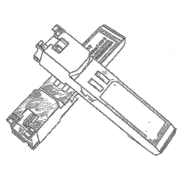 SFP-T (1G/2.5G/10G)
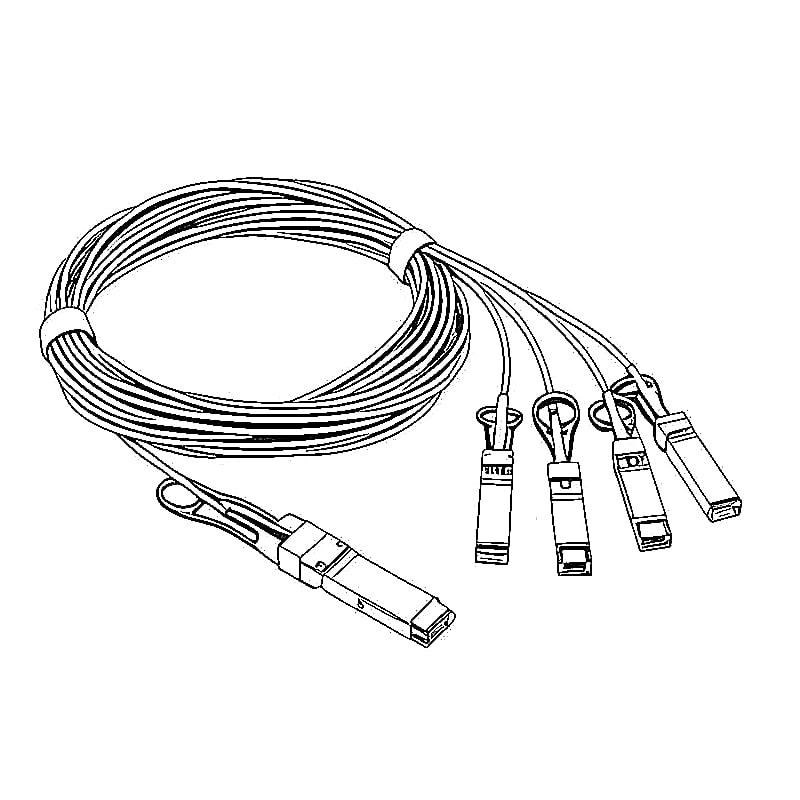
 AOC Cable 10G/25G/40G/100G
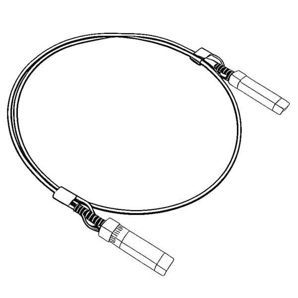 DAC Cable 10G/25G/40G/100G
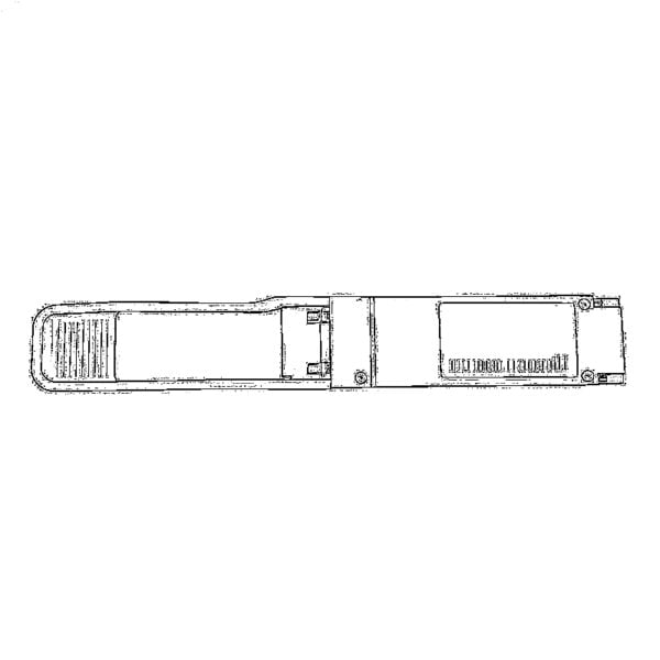 QSFP28 QSFP+ SFP28 100G/40G/25G
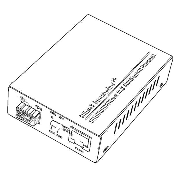
 Copper to Fiber Media Converters
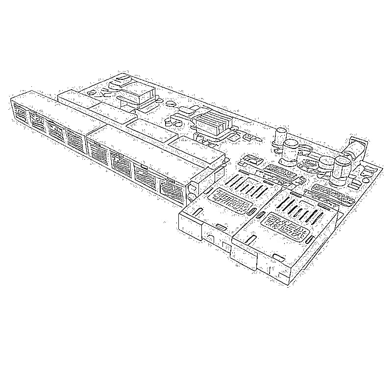
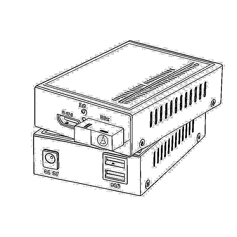
 Fiber Media Converter PCBA Board
 OEO Fiber Media Converters
 Serial to Fiber Media Converters
 Video to Fiber Media Converters
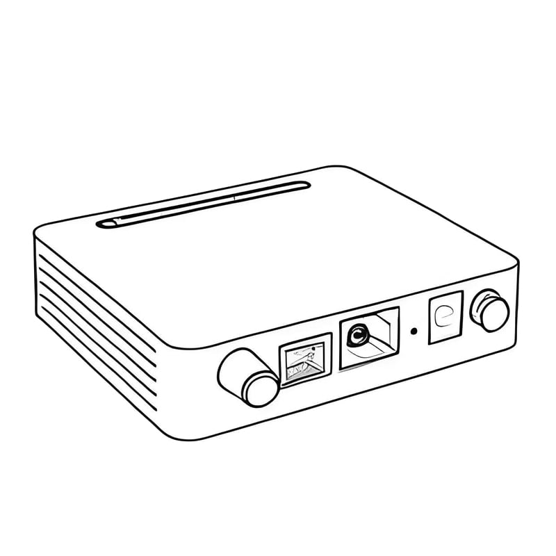
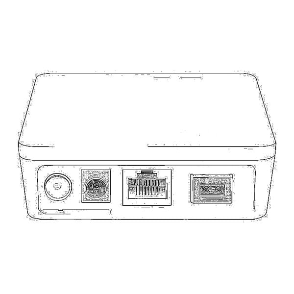 1000M GPON/EPON ONU
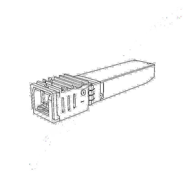 10G EPON ONU/XG-PON/XGS-PON
 2.5G GPON/XPON STICK SFP ONU
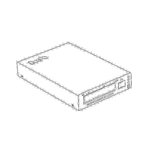 POE GPON/EPON ONU
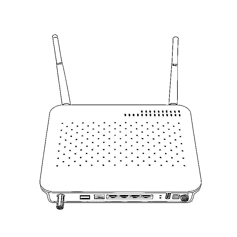
 Wireless GPON/EPON ONT
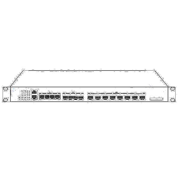 EPON OLT
 GPON OLT
 SFP PON Module
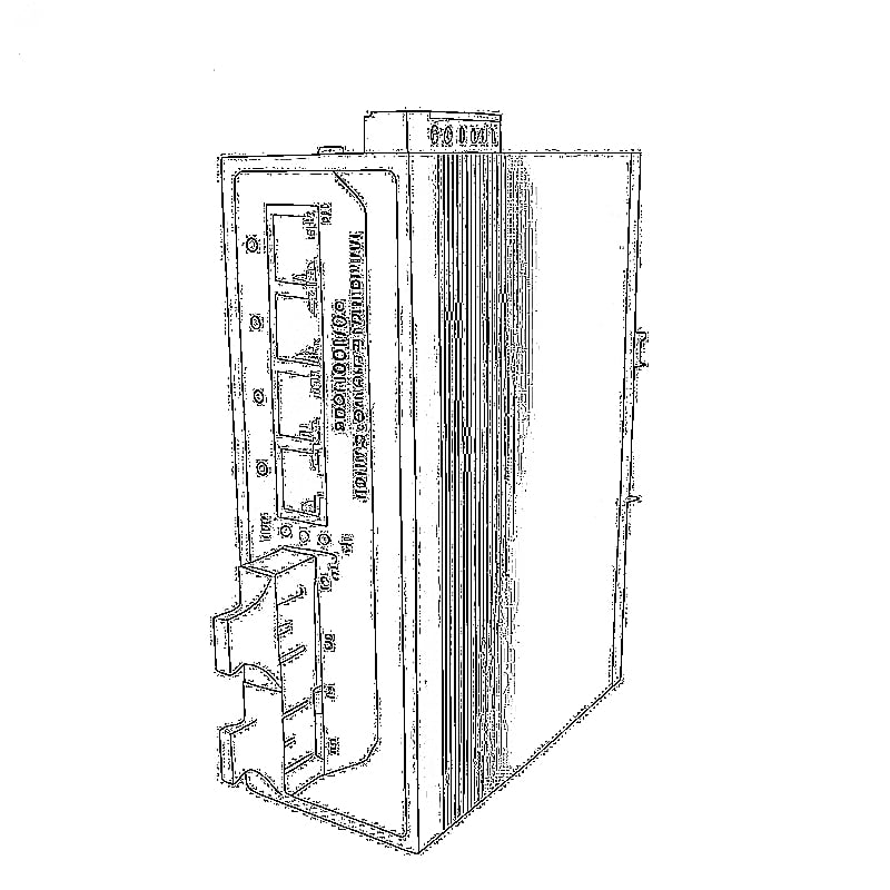
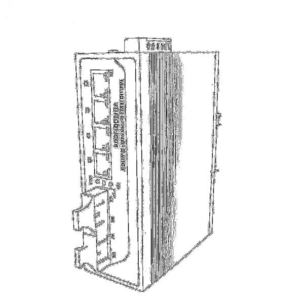 Industrial Switches
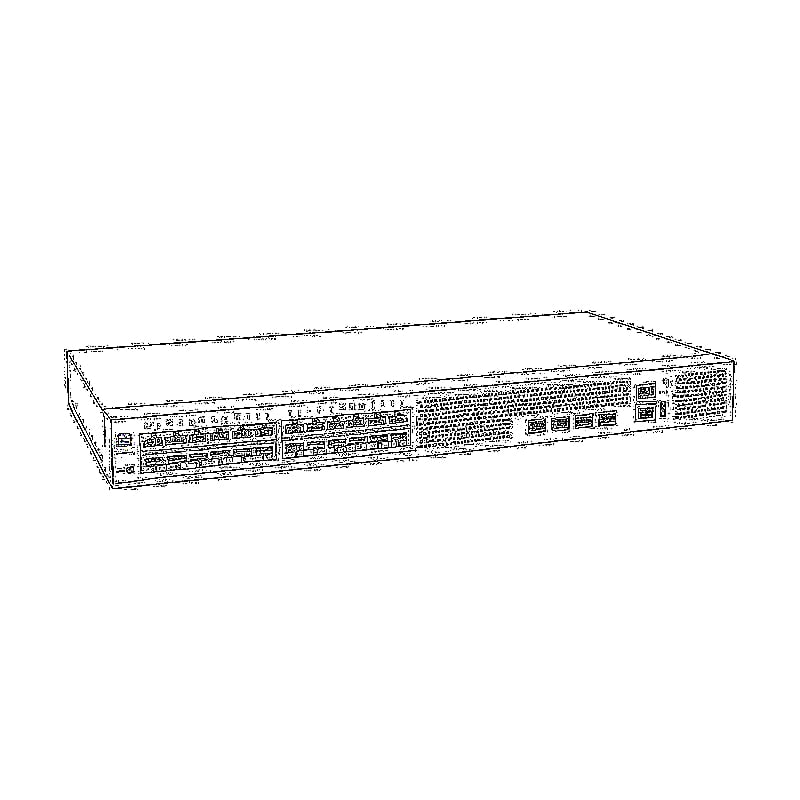
 Managed Switches
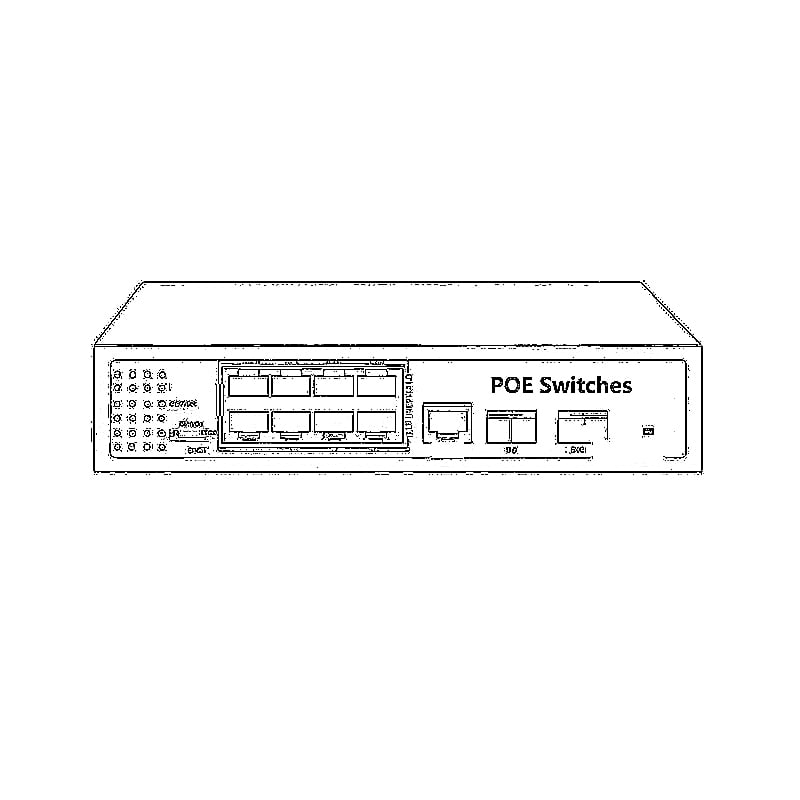
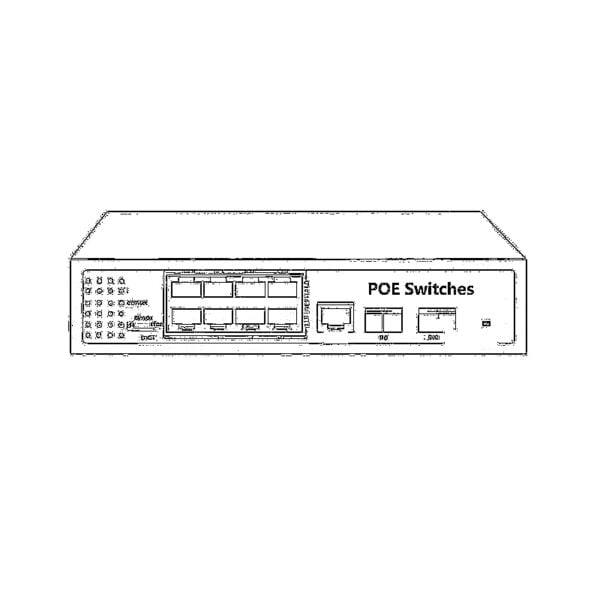 POE Switches
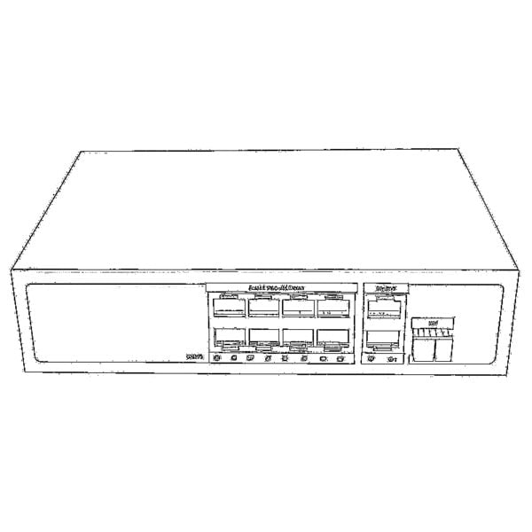 Unmanaged Switches
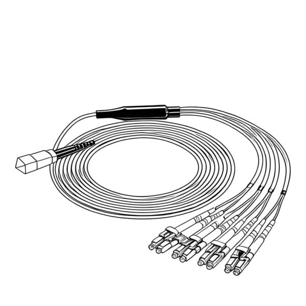 MTP/MPO Fiber Cables
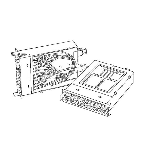 Fiber Optic Cassettes
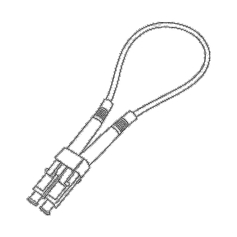
 Fiber Optic Loopback
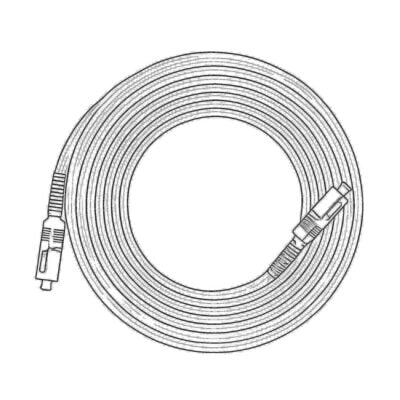 Optic Cables and Fiber Pigtails
 Optical Splitters and Splitter Box
 Fiber Flange Connectors
 Optical Adapters
 Optical Attenuator
 Quick Connector and Connector Panel
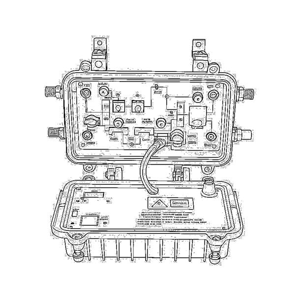
 CATV Amplifier
 CATV Optical Receiver
 Visual Fault Locator
 OTDR
OTDR Optical Power Meter
 Fiber Optic Identifier
 Fiber Optic Cleaners
 Fiber Cleavers & Fiber Strippers
 Copper Tools